Tuesday, January 17, 2012

Installing and Configuring Apache Hadoop for Windows

As has been mentioned in previous posts, I’ve been spending a lot of time recently working with “Big Data” technologies and have been working more recently with Apache Hadoop and associated distributed computing and analytics mechanisms.

What Exactly Is Hadoop?

If you haven’t been exposed to it, Apache Hadoop is an open-source framework that enables distributed processing of very large scale data sets. In a nutshell, Hadoop is comprised of a distributed filesystem, and a framework that allows you to execute distributed MapReduce jobs.

Hadoop has been developed for various flavors of Linux, but is created in such a manner that it can actually run on Windows as long as you have a shell that can support running Linux commands and scripts. While I don’t think anyone would argue that you’d want to do this for a large-scale production environment, running Hadoop on Windows allows folks like me who are very comfortable with installing, using and maintaining Windows servers to also work with exciting technologies such as Hadoop.

The purpose of this post is to demonstrate how you can install and configure a Hadoop cluster using Windows Server 2008 R2. In future posts I’ll demonstrate using Hadoop and the Hadoop Filesystem (HDFS) to perform large-scale analytics on unstructured data (which is what it excels at!)

Preparing to Install Hadoop

The first thing you’ll need to do in order to install Hadoop is to prepare a “virgin” Windows Server. While I suppose it’s not really necessary, from my perspective the fewer things that are installed on the server the better. In my case, I’m using Windows Server 2008 R2 with SP1 installed and nothing else. No roles are enabled and no extra software has been installed.

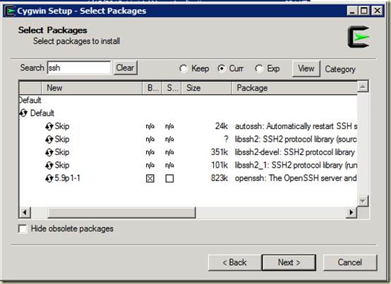
Once you have a server ready (multiple servers if you want to install an actual Hadoop cluster) you’ll want to install Cygwin. If you aren’t familiar, Cygwin is basically a Linux bash shell for Windows. Cygwin is open source and is available as a free download from: http://cygwin.com/install.html Keep in mind that this is just a web installer. To support Hadoop, we will need to ensure that we install the openssh package and it’s associated pre-requisites. In order to do this, start the setup.exe program, select c:\cygwin as the root folder, and then click next. When you get to the screen that asks you to select a package, search for openssl and then click the “skip” (Not exactly intuitive, but it works) text to enable the checkbox for install as shown below:

image

Once you have selected the openssh library, click next and then answer “Yes” when asked if you want to install the package pre-requisites. Click next and then finish the wizard for install. This will take some time, so be patient.

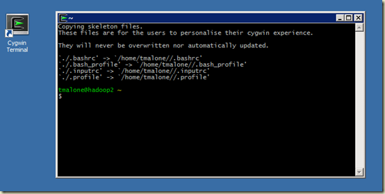
Once the install is complete, you’ll want to start the Cygwin terminal as administrator (right-click on the icon and select “run as administrator”) This will then setup your shell environment as follows:


image

Once Cygwin is installed and running properly, you’ll need to configure the ssh components in order for the hadoop scripts to execute properly.

Configuring Openssh

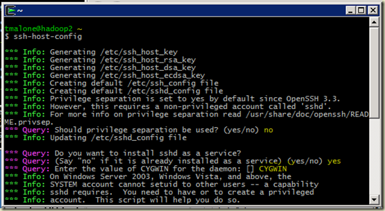
The first step in configuring the ssh server is to run the configuration wizard. Do this by executing ssh-host-config from the cygwin terminal window, which will start the wizard. Answer the questions as follows:

image

(No to Privilege separation, Yes to install as a service, and CYGWIN as the value)

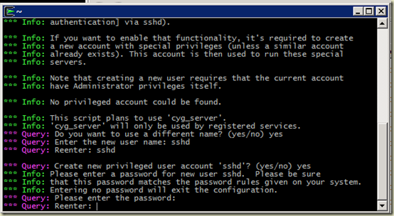
image

(yes to different name, and sshd for the name, yes to new privileged user, and a password you can remember)

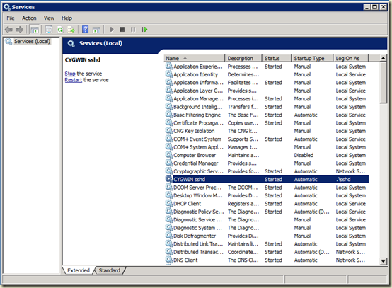
Once the configuration is complete, open the Services control panel (start/administrative tools/services) and right-click on the Cygwin sshd Service and select start. It should start.

image

If the service doesn’t start, the most likely cause is that the ssh user was not created properly. You can manually create the user and then add it to the service startup and it should work just fine.

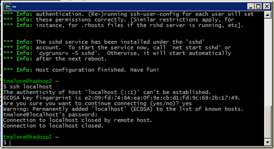
Once the service is started, you can test it by entering the following command in the Cygwin terminal:

ssh localhost

image

Answer “yes” when prompted about the fingerprint, and you should be ready to go.

The next step in configuring ssh for use with Hadoop is to configure the authentication mechanisms (otherwise you’ll be typing your password a lot when running Hadoop commands).

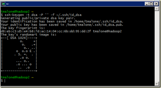
Since the Hadoop processes are all invoked via shell scripts and make use of ssh for all operations on the machine (including local operations), you’ll want to generate key-based authentication that can be used so that ssh doesn’t require the use of a password every time it’s invoked. In order to do this, execute the following command in the Cygwin terminal:

ssh-keygen –t dsa –P ‘’ –f ~/.ssh/id_dsa

image

Once you have the key generated and saved, we’ll need to copy it with the following command:

cat ~/.ssh/id_dsa.pub >> ~/.ssh/authorized_keys

image

This will take the key you just generated and save it to the list of authorized keys for ssh.

Now that ssh is properly configured, you can move on to installing and configuring Hadoop.

Downloading and installing Hadoop

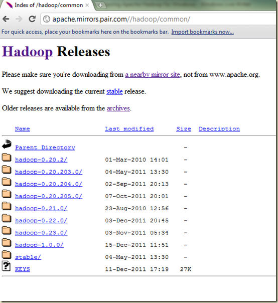
Apache Hadoop is available for download from one of many mirror sites linked from the following page: http://www.apache.org/dyn/closer.cgi/hadoop/common/ 

Basically just choose one of the sites, and it should bring you to a page that looks similar to the following figure. Note that I am going to use version 1.0.0 which as of this writing is the latest, but the release train for hadoop sometimes moves pretty fast, so there will likely be more releases available very soon.

image

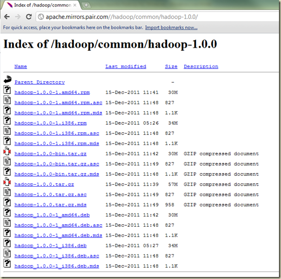
Click on the version you want to install (again, I am going to be using 1.0.0 for this post) and then download the appropriate file. In my case, that will be hadoop-1.0.0-bin.tar.gz as shown in the following figure:

image

Once you have the file downloaded, you’ll want to use a program such as Winrar which can understand the .tar.gz file format.

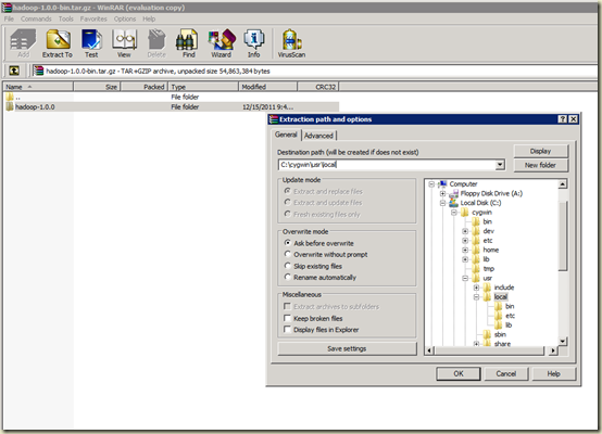
The actual install process is very simple. You simply open the downloaded file in Winrar (or other program that can understand the format) and extract all files to c:\cygwin\usr\local as shown below:

image

Once you are done, you’ll want to rename the c:\cygwin\usr\local\hadoop-1.0.0 folder to hadoop. (This just makes things easier as you’ll see once we start configuring and testing hadoop)

You will also need the latest version of the Java SDK installed, which can be downloaded from http://www.java.com (make sure you download and install the SDK and not the runtime, you’ll need the server JVM) . To make things easier, you can change the target folder for the java install to c:\java (although this is not a requirement – I find it easier to use than the default path, as you’ll have to escape all of the spaces and parens when adding this folder to the configuration files)

Configuring Hadoop

For the purposes of this post, I’m just going to configure a single node Hadoop cluster. This may seem counter-intuitive, but the point here is that we get a single node up and running properly and then we can add additional nodes later.

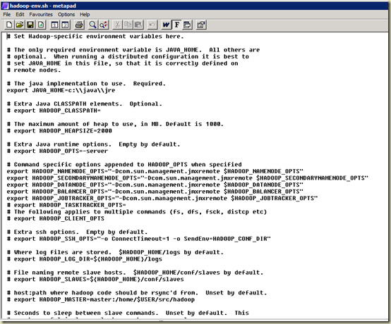
One of the key configuration needs for Hadoop is the location where it can find the Java Runtime. Note that the configuration files we’re going to work with are Unix/Linux files and thus don’t look very good (or work very well) when you use a standard Windows text editor like Notepad. To keep things simple, use a text editor that supports Unix formats such as MetaPad. Assuming that you extracted the Hadoop files as described above and renamed the root folder to Hadoop, open the C:\cygwin\usr\local\hadoop\etc\hadoop\hadoop-env.sh file. Locate the line that contains JAVA_HOME, remove the # in front of it, and replace the folder with the location you installed the Java sdk (in my example, C:\java\jre. (Note that this is a Unix file, so special characters must be escaped with a “\”, so in my case the path is c:\\java\\jre).

image

This is really all that is required to change in this file, but if you want to know more about the contents you can check out the Hadoop documentation here: http://hadoop.apache.org/common/docs/r0.20.2/quickstart.html (Note that this guide is based on the 0.20.2 release and *not* the 1.0.0 release I detailing here. The docs haven’t quite caught up with the release at the time of this posting)

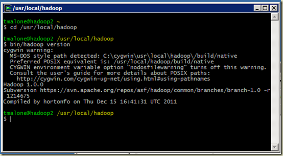
Once you save and close that file, you can verify that Hadoop is properly running by executing the following command inside of Cygwin. (Make sure you change to the /usr/local/hadoop directory first)

bin/hadoop version

image

You should see a Cygwin warning about MSDOS file paths, and then a version of Hadoop and Subversion located as shown in the figure above. If you do not see a similar output, you likely do not have the path to your Java home set correctly. If you installed Java in the default path, remember that all spaces, slashes and parens must be escaped first. The default path would look like: C:\\Program\ Files\ \(x86\)\\Javaxxxx (you get the idea and probably understand now why I said it would be better to put it in a simple folder)

Once you have the basic Hadoop configuration working, the next step is to configure the site environment settings. This is done via the C:\cygwin\usr\local\hadoop\etc\hadoop\hdfs-site.xml file. Again open this file with MetaPad or a similar editor, and add the following configuration items to the file. Of course replace “hadoop2” with your host name as appropriate:

<?xml version="1.0" encoding="utf-8"?>
<?
xml-stylesheet type="text/xsl" href="configuration.xsl"?>
<!--
Put site-specific property overrides in this file. -->
<
configuration>
<
property>
<
name>fs.default.name</name>
<
value>hdfs://hadoop2:47110</value>
</
property>
<
property>
<
name>mapred.job.tracker</name>
<
value>hadoop2:47111</value>
</
property>
<
property>
<
name>dfs.replication</name>
<
value>2</value>
</
property>
</
configuration>


This basically configures the local host (in my case it’s named hadoop2) filesystem and job tracker, and sets the dfs replication to 2 blocks. You can read about this file and it’s values here: http://wiki.apache.org/hadoop/HowToConfigure (again remember that the docs are outdated for my particular installation, but they still work)


We will also need to configure the mapred-site.xml file to specify the configuration for the mapreduce service:


<?xml version="1.0"?>
<?
xml-stylesheet type="text/xsl" href="configuration.xsl"?>

<!--
Put site-specific property overrides in this file. -->

<
configuration>
<
property>

<
name>mapred.job.tracker</name>
<
value>hadoop2:8021</value>
</
property>
</
configuration>


This basically configures the mapreduce job tracker to use port 8021 on the local host. There is a LOT more to both of these configuration files, I’m only presenting the basics to get things up and running here.


Now that we have the basic environment setup, we need to format the HDFS filesystem that Hadoop will use. In the configuration file above, I did not specify a location for the DFS files. This means that they will be stored in /tmp. This is OK for our testing and for a small cluster, but for production systems  you’ll want to make sure that you specify the location by using the dfs.name.dir and dfs.data.dir configuration items (which you can read about in the link I provided above).


To format the filesystem, enter the following command in cygwin:


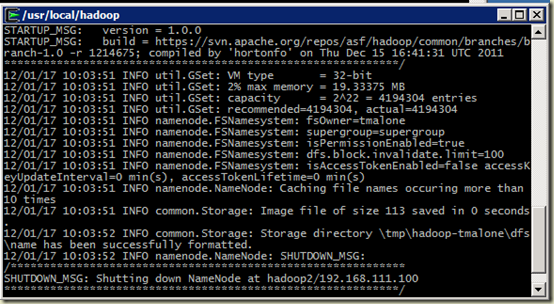
bin\hadoop namenode –format


image


If you have properly configured the hdfs-site xml file, you should see output that is similar to the above. Note in my case that the default folder location is /tmp/hadoop-tmalone/dfs/name. Remember this directory name as you will need it later.


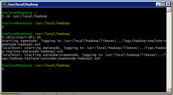
Now that we have the configuration in place and the filesystem formatted, we can start the Hadoop subsystems. The first thing we’ll want to do is start the DFS subsystem. Do this with the following command in the Cygwin terminal:


sbin/start-dfs.sh


image


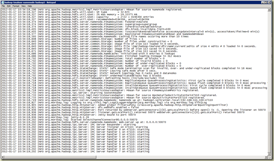
This should take a few moments, and you should see output as shown in the figure above. Note that the logs are stored in /usr/local/hadoop/logs. You can verify that DFS is running by examining the namenode log:


image


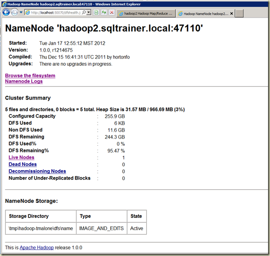
You can also verify that the DFS service is running by checking the monitor (assuming you used the ports as I described them in the hdfs-site xml configuration above). To check the monitor, open a web browser and navigate to the following site:


http://localhost:50070


image


If the DFS service is properly running, you will see a status screen like the above. If you get an error when attempting to open that page, it is likely that DFS is not running and you will need to check the log file to determine what has gone wrong. Most common problem is a misconfiguration of the site-xml file, so double check that the file is correct.


Once DFS is up and running, you can start the mapreduce process as follows:


sbin/start-mapred.sh


image


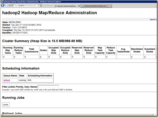
You can test that the Mapreduce process is running by checking the monitor. Open a web browser and navigate to:


http://localhost:50030


image


Now we have success! We’ve installed and configured Hadoop, formatted the DFS filesystem, and started the basic processes necessary to use the power of Hadoop for processing!


Testing the installation


Each Hadoop distribution comes with a set of samples that can be used to very that the system is functional. The samples are stored in Java “jar” files and are located in the hadoop/share/hadoop directory. One simplistic test would be to copy some text files into DFS and then use the sample mapreduce job to enumerate them. First though, you will likely want to setup an alias to make entering the commands a little easier. In my case, I will alias the hadoop dfs command to simply “hdfs”. Do accomplish this, type the following command in the Cygwin terminal window:


alias hdfs=”bin/hadoop dfs”


image


For the first part of our test, we will copy the configuration files from the hadoop directory into DFS. In order to do this, we will use the dfs –put command (for more information on the put command, see the docs here: http://hadoop.apache.org/common/docs/r0.20.0/hdfs_shell.html (again remember that the docs are a little behind)


In the Cygwin terminal window (still in the /usr/local/hadoop directory) execute the following command:


hdfs –put etc/hadoop conf


image


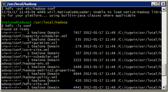
This will load all of the files in the /usr/local/hadoop/etc/hadoop directory into HDFS in the conf folder. Since the conf folder doesn’t exist, the –put command will create it. Note that you receive a warning about the platform, but that is OK the files will still copy.


You can verify that the files were copied by using the dfs –ls command as follows:


hdfs –ls conf


image


Now that we are sure the files are stored in HDFS, we can use one of the examples that is shipped with Hadoop to analyze the text in the files for a certain pattern. The samples are located in the /usr/local/hadoop/share/hadoop folder, and it’s easiest to change to that folder and execute the sample there. In the Cygwin terminal, execute the following command:


cd /usr/local/hadoop/share/hadoop


Once we’re in the folder, we can run a simple IO test to determine how well our cluster DFS IO will perform. In my case, since I’m running this on a VM with a slow disk, I don’t expect much out of the cluster, but it’s a very nice way to test to see that DFS is indeed functioning as it should. Execute the following command to test DFS IO:


../../bin/hadoop jar hadoop-test-1.0.0.jar testDFSIO –write –nrFiles 10 –filesize 1000


image


If you don’t see any exceptions in the output, you have successfully configured Hadoop and the DFS cluster is operational.


Conclusion


While it isn’t exactly a simple process, you can indeed get Apache Hadoop up and running on a Windows platform. I’ve taken the path of configuring Hadoop with Cgwin as the shell, but there are those who claim to have installed and configured Hadoop on windows without the use of Cygwin. Either way, I’m just glad it works and folks who don’t want to invest in building a Linux environment have the ability to play around with and use Hadoop.
Friday, December 30, 2011

Fun with Decision Trees using R and SQL Server

As those who have been reading this blog know, I’ve recently been spending a lot of time doing statistical analysis with R and SQL Server and have really been enjoying digging in to the various bits of functionality that is offered.

One thing I’ve learned over the years is that I am a very “classification-oriented” individual when it comes to working with data. I work best with data sets that I understand and that I’ve been able to sort into the various buckets that make sense to me based on what I’m trying to accomplish with the data.

The problem with this need for nice and tidy data classification is that it doesn’t work well when you don’t really have a complete understanding of the data set you’re working with. This especially becomes an issue if you’re trying to mine the data you have in order to predict future outcomes based on past performance (a requirement that is becoming more and more importing to “Data Scientists” as more and more organizations make that shift to true data-driven processes.

Understanding Data

If you read my previous post on creating a large SQL Server database, you’ve seen some of the data that I am playing around with. Obviously there is a lot of interesting information locked within the mortgage loan application data stored in the HMDA database. One specific use-case with this data might be to look at some of the deciding factors related to home loans being granted and create some predictive models based on the data. For example, I might want to predict the outcome of a home loan application process based on factors like the purpose of the loan, the income of the applicant, and some other factors such as race. This could be very useful for a mortgage company to look at and see who to target for an ad campaign, or maybe to research things such as do race or sex have any correlation to the amount of a home loan given. In order to answer this use case, we need to have a good understanding of the data we’re working with and see what it looks like when shaped into a “Decision Tree” (for more information on what exactly a decision tree is, take a look at: http://en.wikipedia.org/wiki/Decision_tree )

Creating a Data Set to Work With

If we wanted to use the home mortgage disclosure data to look at past performance of home loans, the first thing we need to do is create a manageable data set to use to create a model. Since I live in El Paso County, Colorado, I’ll create a table of data that just details information on Home Loans in this area. Given the database that was created earlier (see previous post) We can create a subset of the data with the following query:

SELECT 
loan_purpose AS [purpose]
,loan_amount AS [amount]
,CASE WHEN applicant_race = 'White' THEN applicant_race ELSE 'Non-White' END AS [race]
,applicant_sex AS [sex]
,applicant_income AS [income]
,CASE WHEN denial_reason = 'Approved' THEN denial_reason ELSE 'Denied' END AS [status]
INTO
tblElPasoCountyLoanStatus
FROM
vColoradoLoans
WHERE county='El Paso County'


What this will do is create a simple table that has 6 columns. I’ve simplified the data slightly so that some of the factors (race, denial reason) are binary values as opposed to continuous. While this is not a necessary transformation for the most part, it helps simplify the output for the purposes of this discussion.


Loading the Appropriate Packages and Libraries in R


Once I’ve created the table above in SQL Server, I can load the data into R and begin analysis. Before we get too deep in the creation of the decision tree, I should mention that I am going to use a package called “rpart” as well as a package called “rpart.plot”. If you are really curious and would like to know the science behind the rpart package, there is a very dry document here that explains the algorithm in detail: http://www.mayo.edu/hsr/techrpt/61.pdf 


The rpart package can be found here: http://cran.stat.ucla.edu/web/packages/rpart/index.html


and rpart.plot can be found here: http://cran.stat.ucla.edu/web/packages/rpart.plot/index.html 


Of course you really don’t need to know where exactly the packages are, you can install them with the R command as follows:


image


When you execute the above command in the R console, you will be prompted for the mirror site you wish to use, and the package will be downloaded, unpacked and installed. Once the packages are installed, you can load them into your R environment as follows:


image


Connecting to SQL Server Data


Once the libraries are loaded, we need to obtain the data we’re going to work with. If you haven’t worked with SQL Server data in R before, you might want to read my previous post on connecting R to SQL Server via the ODBC library. First we need to setup an ODBC channel to connect to the table we created above. Is is done via the following command:


image


(Remember that “HMDAData” is the name of the ODBC DSN I created to connect to my database)


Once the channel is created, I can load the data from the table via the sqlFetch command in R as follows:


image


Examining the Data


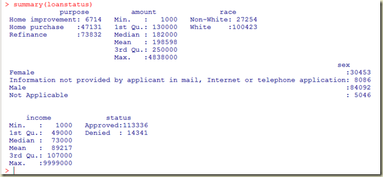
This loads the data from the table into the R variable “loanstatus”. You can view a summary of the loanstatus as follows:


image


Already you can see that we’ve extracted some good information out of the database. (as a side note here, I think this is VERY COOL! Think of all the SQL Queries I’d have to run to get this same information from the table I created earlier)


Now that we have the data in an R variable, we can start to create a decision tree. Since we ultimately want to use this data to predict the amount of a loan based on certain factors such as race, sex and income, we’ll create a regression tree shaped to those parameters. We will use the rpart function in order to create the tree. rpart is a very simplistic function that accepts the following parameters:


  • formula – The formula is specified in the following format: outcome ~ predictor1 + predictor2 + predictor3 etc.


  • data – The specific data frame to use


  • method – “class” for a classification tree or “anova” for a regression tree


Remember that within R, you can always type ? <function> to get a full description of a particular function.


In our case, the rpart command would look like this:


image


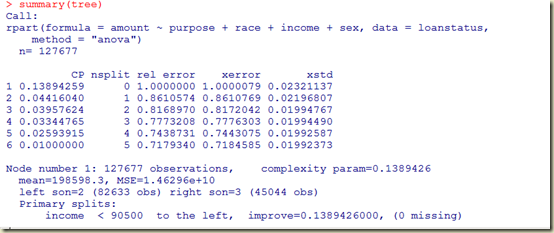
Once we’ve created the tree variable (this can be named anything, I just kept it simple and named it “tree” here) we can look at a summary and determine what it looks like:


image


(there are a total of 13 nodes in my specific example, and I can’t paste the entire tree here in text form)


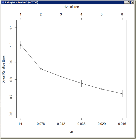
One big factor in determining how useful a particular decision tree going to be is to examine the “complexity parameter” (“cp” for short) for each of the nodes. The CP is used to cross-validate the data and make sure that the tree is pruned to remove the portions of the tree that are “over fitted” (You can read about the terminology here: http://www.statmethods.net/advstats/cart.html ) . Since I am a very visual person, I like to see this cross-validation data in chart form as follows:


image


Which generates a nice graph showing me the relative size of the tree, the cross-validated error that is generated, and the resulting cp:


image


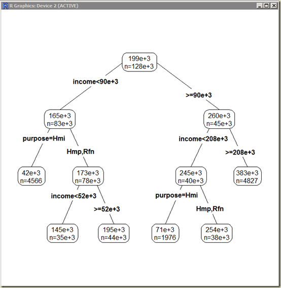
Since the tree that I am working with is relatively small, I am not going to worry about pruning it here and removing the “bad” cp values. To generate the decision tree, use the following command:


image


(Remember that you can use the ? command to get a full listing of all options for a given function. In this case, by using type=4 I am instructing R to generate a plot containing all nodes and all information, and by using extra=1 I am instructing R to include the number of nodes in each branch)


image


With this visual of the tree, I can see that income seems to be a deciding factor, and it splits at approximately 90,000. Following the tree to the left, for those with less than 90K income, we see a split for Home Improvement loans versus Home Purchase and refinance. For the purchase and refinance, we see another split at approximately 52K income. Back on the right side of the tree we see a split at approximately 208K income, with the same split for home improvement loans versus purchase and refinance.


Conclusion


Being the data geek that I am, I could continually refine this model and graph it to start finding the patterns and determining just exactly how the data is shaped. At that point I could feed additional data into the model and use it to predict outcomes based on past performance. There are many things that can be done with Decision Trees and I’ve only scratched the surface here with this post. I’ll be writing many more of these posts in the future as I continue to explore the magic of data mining with R.

Wednesday, December 28, 2011

To The Cloud and Back Again! – SQL Saturday # 104

For those that are not aware, the Professional Association for SQL Server (PASS) has chapters throughout the world that put on one day events called “SQL Saturday”. As the name implies, these events take place on a Saturday and generally are a full day of targeted learning for those who want to know more about SQL Server and SQL Server technologies.

This year, the first US SQL Saturday event (There is also an event in Bangalore that same day, and given the time zones, I’d say they qualify as the “first” one of the year!)  is happening right here in Colorado Springs! SQL Saturday #104 has a very distinguished list of speakers, including people like Jason Horner, TJ Belt, Chris Shaw, Thomas LaRock, Karen Lopez and a whole host of very impressive speakers. There’s going to be 5 simultaneous tracks and somehow they even invited me to speak as well, so I’ll be speaking at 0830 in room #4 on “To the Cloud and Back Again!”.

Session Description

In this session, I’ll be introducing some basic Cloud Computing patterns and will talk about some specific cloud computing security concerns. I’ll then talk about some of the specific technologies that accompany the Windows Azure and SQL Azure platforms that enable a hybrid approach to cloud computing. I’ll demonstrate how Windows Azure roles can be “Domain Joined” that will then allow Azure-based applications to use SQL Server Trusted Connections to connect to on-premises SQL Server databases. All in all I hope it will be a very informative session on Cloud Computing technologies. Hope to see you there!

image

Monday, December 26, 2011

Building a large real-world SQL Server demo database

In my previous post, I discussed a large data set that I was using for demonstrations and working with R. Instead of using the normal AdventureWorks or Northwind databases that Microsoft makes available to us via Codeplex, I wanted something a bit more real-world as well as large. I also wanted something that I could continue to build on as more data became available. I had never really found anything that I liked and basically relegated the thought to a background task.

As I mentioned in the last post,  I had the opportunity to attend an alpha delivery of the EMC “Data Science and Big Data Analytics” training course. As we were working through the labs, I couldn’t help but think that the data set being used was very interesting, and would almost fit what I had been looking for. In speaking with the creators of the class, I learned that they had built the database based on information obtained from the publically-available “Home Mortgage Disclosure Act” reporting site. Here in the US, when you apply for a home mortgage loan you must provide certain information to the lending institution, and they in turn must report information on all applications that they process, whether they are approved or denied. The information itself is stripped of personal-identifiers when it is submitted, but the overall type of data that is reported is extremely interesting from both a volume perspective as well as a content perspective. I decided to spend a bit of time looking in to how I could gain access to this data, and thanks to the magic of the interwebs, I was able to piece together everything I needed in order to build the database I was looking for.

Gaining Access to the Home Mortgage Disclosure Act Data

(I realize that the information posted here is really only relevant to those of us in the United States, however I believe the resulting data is useful and relevant worldwide for purposes of learning or demo)

The Home Mortgage Disclosure Act was enacted by Congress in 1975 and is administered by the “Federal Financial Institution Examination Council”. Because it is a government institution and funded by US taxpayer dollars, the data that they collect and maintain is made available to the public free of charge. Basically what they do is chunk the data into yearly “drops” that are made available according to a specific timeline. You can read about the timeline here: http://www.ffiec.gov/hmda/timeline.htm 

The data itself is available from the following link:

http://www.ffiec.gov/hmda/

There are multiple ways to obtain the data for a given year. The easiest way to get to the data is to download the “LAR/TS Windows Application” for a given year. (LAR = “Loan Accounts Register”, TS=”Transmittal Sheet”). You can download the application from the following link: http://www.ffiec.gov/hmda/hmdaproducts.htm (note the Windows application download links towards the bottom of the page). When downloaded, the application contains all of the data for a given year within a SQL Server Compact Edition (SQLCE) database. The database itself is about 5GB per year. Of course the problem with this format is that it’s strictly a SQLCE database, which means you’ll want to extract the data for use with SQL Server. Another issue with the data is that it is organized by a seemingly random collection of states, meaning that there is no single dataset that contains the data within a given year for the entire country.

Another way to obtain the data is to download the text files directly from the site. The files are zipped and can be found by downloading the “ALL” file in the LAR table for the year that you are interested in. (At the time of this posting, there are 3 years available, 2008, 2009 and 2010). These files are tab-delimited and will need to be imported to SQL Server.

Creating the HMDA Database

Because I want to create a database that will have a single “fact” table containing all of the LAR records, I will need to first create the database and then the table structure necessary. The HMDA data is very “flat” and denormalized, so it works very well as a fact table. There are 45 fields contained in the text file and column names are NOT included in the first row. The data dictionary can be found here: LAR Record Format

Since the resulting database will work out to be about 5GB per year, and since we’ll be importing 3 years of data, I’ll start by creating a 15GB database with the following T-SQL(I am using SQL Server 2012 as my destination, so some of the syntax might be slightly different than you are used to) command:

CREATE DATABASE [HMDAData]
CONTAINMENT = NONE
ON  PRIMARY
( NAME = N'HMDAData', FILENAME = N'C:\SQLData\MDF\HMDAData.mdf' , SIZE = 15GB , MAXSIZE = UNLIMITED, FILEGROWTH = 1024MB )
LOG ON
( NAME = N'HMDAData_log', FILENAME = N'C:\SQLData\LDF\HMDAData_log.ldf' , SIZE = 8GB , MAXSIZE = 2048GB , FILEGROWTH = 10%);

Once the database is created, we can create the table to hold the LAR records. The table can be created with the following command:


CREATE TABLE [dbo].[lar_data](
    [year] [int] NOT NULL,
    [respid] [nchar](10) NOT NULL,
    [agycd] [nchar](1) NOT NULL,
    [loan_type] [int] NOT NULL,
    [property_type] [int] NOT NULL,
    [loan_purpose] [nchar](1) NULL,
    [occupancy] [nchar](1) NULL,
    [loan_amount] [nchar](5) NULL,
    [preapproval] [nchar](1) NULL,
    [action_type] [nchar](1) NULL,
    [msa_md] [nchar](5) NULL,
    [state_code] [int] NOT NULL,
    [county_code] [int] NULL,
    [tract_code] [nchar](7) NOT NULL,
    [applicant_ethnicity] [nchar](1) NULL,
    [co_applicant_ethnicity] [nchar](1) NULL,
    [applicant_race_1] [nchar](1) NULL,
    [applicant_race_2] [nchar](1) NULL,
    [applicant_race_3] [nchar](1) NULL,
    [applicant_race_4] [nchar](1) NULL,
    [applicant_race_5] [nchar](1) NULL,
    [co_applicant_race_1] [nchar](1) NULL,
    [co_applicant_race_2] [nchar](1) NULL,
    [co_applicant_race_3] [nchar](1) NULL,
    [co_applicant_race_4] [nchar](1) NULL,
    [co_applicant_race_5] [nchar](1) NULL,
    [applicant_sex] [nchar](1) NULL,
    [co_applicant_sex] [nchar](1) NULL,
    [applicant_income] [nchar](4) NULL,
    [purchaser_type] [nchar](1) NULL,
    [denial_reason_1] [nchar](1) NULL,
    [denial_reason_2] [nchar](1) NULL,
    [denial_reason_3] [nchar](1) NULL,
    [rate_spread] [nchar](5) NULL,
    [HOEPA_status] [nchar](1) NULL,
    [lien_status] [nchar](1) NULL,
    [edit_status] [nchar](1) NULL,
    [seq_number] [nchar](7) NULL,
    [population] [int] NULL,
    [minority_population_percent] [numeric](18, 0) NULL,
    [median_income] [int] NULL,
    [tract_msa_income_percent] [numeric](18, 0) NULL,
    [owner_occ_units] [int] NULL,
    [owner_occ_1_to_4_family] [int] NULL,
    [app_date_pre_2004] [nchar](1) NULL
) ON [PRIMARY];

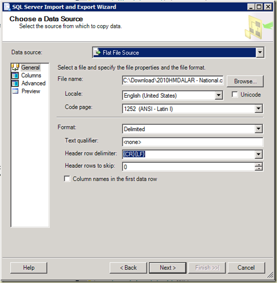
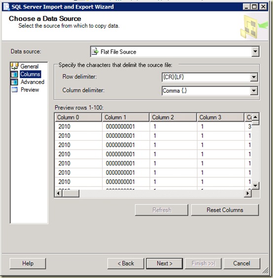
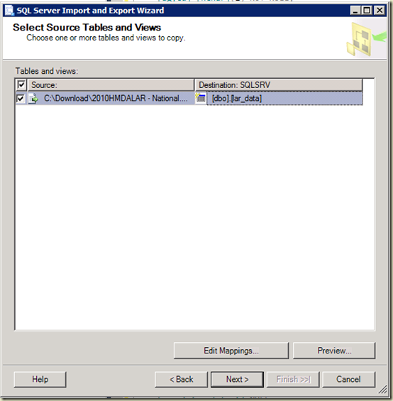
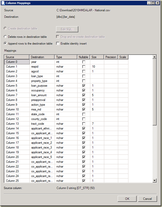
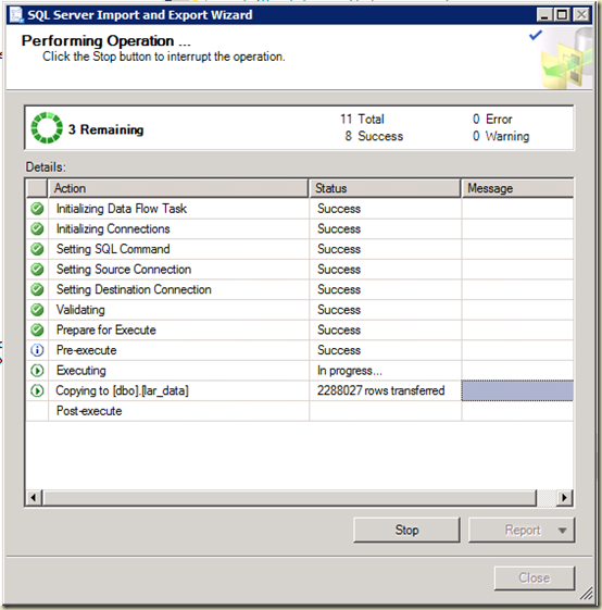
Once the table is created, you can either use the SQL Server Import/Export wizard or SSIS to import each of the files to the lar_data table. Since it is a simple data load process without any conversions needed, the Import/Export Wizard works just fine. Here’s an example of importing the 2010 file to the lar_data table:

image

image

image


image

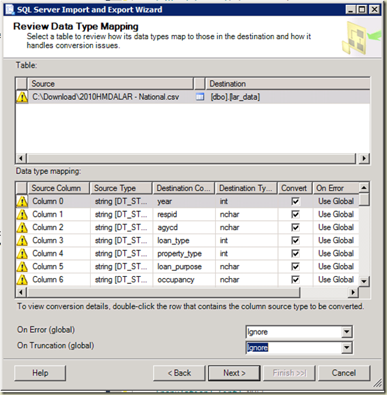
Because the text file will contain character data there will be CASTs required for most columns. In the event that an error occurs within a specific CAST, it’s best to just ignore it. We’re not trying to create a perfect database, just one that works for most conditions.

image

image

When the import for 2010 is complete, there will be approximately 16.3 million rows of data inserted into the table.

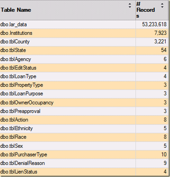
To complete the task, import the remaining years into the table. You should end up with approximately 53.2 million rows in the table if you copy 2008, 2009 and 2010 data.

You may notice that several of the columns are codes and not well described. You can find the information for each of the columns in the data dictionary linked above, however the data for each of the columns can be a pain to enter. Since I have already extracted the data and created appropriate tables, you can download the following ZIP file (which contains text files that are in .csv format with column names as the first row and the file is named the same as the table it comes from. These files are simple to import using the Import/Export wizard. There is also a .sql file there to create the remaining tables and insert descriptive data):

Zip file containing dimension tables and descriptive data

Creating an Appropriate “State” View

Now that you have the fact table data loaded, and you’ve used the files I’ve supplied to create the dimensional tables, you’ll likely want to create a subset of the data for specific analysis. Since I live in Colorado, I decided to create a view that shows only Colorado data. The view definition is included below, and you can modify it accordingly to isolate the data for the state you are interested in:

CREATE VIEW [dbo].[vColoradoLoans]
AS
SELECT
    lt.description AS [loan_type]
    ,lpt.description AS [property_type]
    ,lp.description AS [loan_purpose]
    ,o.description AS [occupancy_type]
    ,CAST(loan_amount AS money) * 1000 AS [loan_amount]   
    ,p.description AS [preapproval]
    ,at.description AS [action_taken]
    ,s.state_name AS [state]
    ,c.county_name AS [county]
    ,e.description AS [applicant_ethnicity]   
    ,r.description AS [applicant_race]
    ,sx.description AS [applicant_sex]
    ,CAST(applicant_income AS money) * 1000 AS [applicant_income]   
    ,pt.description AS [purchaser_type]
    ,dr.description AS [denial_reason]
    ,CASE WHEN rate_spread = 'NA' then 0 ELSE CAST(rate_spread AS numeric) END AS [rate_spread]    
    ,population AS [tract_population]
    ,minority_population_percent
    ,median_income
    ,owner_occ_units
FROM
    lar_data ld
JOIN
    tblLoanType lt
ON
    ld.loan_type = lt.loan_type
JOIN
    tblPropertyType lpt
ON
    ld.property_type = lpt.property_type
JOIN
    tblLoanPurpose lp
ON
    ld.loan_purpose = lp.loan_purpose
JOIN
    tblOwnerOccupancy o
ON
    ld.occupancy = o.owner_occupancy
JOIN
    tblPreapproval p
ON
    ld.preapproval = p.preapproval
JOIN
    tblAction at
ON
    ld.action_type = at.action_taken
JOIN
    tblState s
ON
    ld.state_code = s.state_code
JOIN
    tblCounty c
ON
    ld.county_code = c.county_code AND s.state_name=c.state_name
JOIN
    tblEthnicity e
ON
    ld.applicant_ethnicity = e.ethnicity
JOIN
    tblRace r
ON
    ld.applicant_race_1 = r.race
JOIN
    tblSex sx
ON
    ld.applicant_sex = sx.sex
JOIN
    tblPurchaserType pt
ON
    ld.purchaser_type = pt.purchaser_type
JOIN
    tblDenialReason dr
ON
    ld.denial_reason_1 = dr.reason
WHERE
    ld.state_code = '08' -- Colorado
AND
    ld.property_type = 1 -- Single Family Homes
AND
    ld.applicant_income <> 'NA' -- remove invalid income reports
;

Conclusion

Once you have the view in place, you now have a very flexible large database that you can use that has a real-world use-case and can be used for demos, performance tuning work, statistical analysis, etc.. Of course you’ll want to add your own indexes and possibly partitions depending on your use case.

image

I know that I’ve often wanted such a database when presenting or demonstrating specific functions within SQL Server, so I hope this database proves useful.

Friday, December 23, 2011

Statistical Analysis with R and Microsoft SQL Server 2012

It’s been awhile since I’ve written a blog post, but that doesn’t mean that I haven’t been thinking about things to write about and discuss here. Recently, I had the opportunity to attend an alpha delivery of EMCs “Data Science and Big Data Analytics” course (Read about the course on EMC Education Services site here: http://education.emc.com/guest/campaign/data_science.aspx ) and was really taken by a couple of points that the course brought home:

1) There’s much more to statistical analysis than I had ever thought about. (Being a Microsoft SQL Server and Microsoft BI Stack kinda guy, I always figured that you needed Excel and SSAS to do real statistical analysis.

2) Big Data Analytics is a really cool technology discipline!

The course itself was based on the EMC Greenplum Database (Community Edition, which you can download and use for free!) which is an amazing piece of technology (I am very impressed with it’s feature/functionality and integration with things like Hadoop for real parallel computing capabilities) as well as the open source “R” statistical analysis language.

R logo

While it’s true that my role at EMC means that I focus more on the non-Microsoft stack these days, that doesn’t stop me from thinking about how I can apply things that I lean to the Microsoft platform. With that in mind, one of the things that I kept coming back to in the class was, “How would I do this using SQL Server?" As it turns out using R with SQL Server isn’t all that difficult, and it really does open up an entirely new way of thinking about statistical analysis (for me anyway)

R and Statistical Analysis

R is an open source “software environment” that is used primarily for statistical analysis. A huge part of “Data Science” is of course statistical analysis, so the two go hand-in-hand. One very cool aspect of R is the fact that the graphics environment is “built in” (I put that in quotes because R is very modular and requires you to load packages for just about anything you do, although a basic “plot” command is included in the base distribution) and allows you not only to analyze data, but also visualize it “on the fly” as well. You can read about (and download) R from the main website here: http://www.r-project.org/. If you are really interested in R, you should make a point of reading the R Journal here: http://journal.r-project.org/current.html 

One thing that is very clear though about R is that it’s a “data source agnostic” environment, but many of the examples that use data either deal with flat files or connect to open source databases like MySQL or Postgres. This of course doesn’t mean you can’t use R with SQL Server, it just means you have to dig a little deeper and understand how to connect the R environment to your SQL Server database.

R and SQL Server

Once you download and install the R environment (the screen shots and examples I provide here will be from the Windows version of RGUI version 2.14.0 which I downloaded from the UC Berkeley mirror here: http://cran.cnr.berkeley.edu/ ) you will need to install the RGUI environment and decide whether you will use the 32 or 64-bit client. This is a very important distinction, since R connects to databases via ODBC, and ODBC drivers are very platform (32 versus 64 bit) specific.

In my case, I am going to use the 64 bit GUI and will be using SQL Native Client 11 to connect to SQL Server 2012. (There is no specific reason for me to use SQL Server 2012 here, other than I’ve been playing around with the release candidate and my development environment is all setup for it) I have a large database that I use for “big data” type demonstrations that also works well for statistical analysis work. I will likely write another article on how this database was constructed, but know that the data is very real world (it is built from 2010 data collected via the US Home Mortgage Disclosure Act) and well-suited for testing statistical analysis theories and data mining.

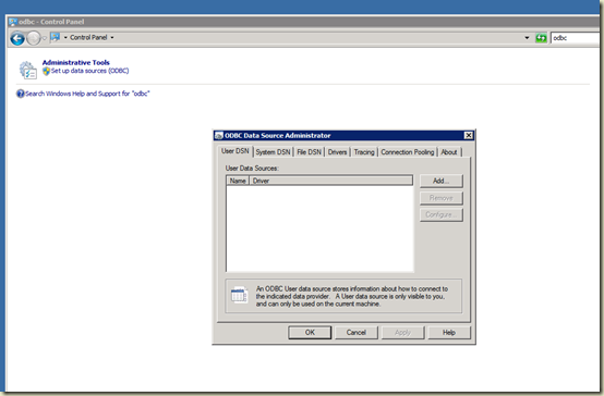
Once you decide what client you will be using, you will need to configure an ODBC DSN (I decided to use a System DSN for my work, so I’ll walk though the creation of that DSN) to connect to your database. To create a new DSN, use the platform-specific version of the ODBC control panel (for Windows Server 2008 R2, simply go to control panel and search for “ODBC”, you will then see the “Set up data sources (ODBC)” as shown in the following figure:

image

Click the “System DSN” tab, and then click the Add button and walk through the wizard to connect to your database. Remember the name of the DSN you create, as you’ll need to specify it from within R in order to connect. In my case, the DSN is named “HMDAData”.

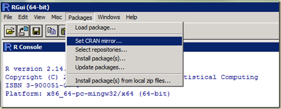
In order to use the ODBC connection within R, you’ll need to download the “RODBC” library, which can be found here: http://cran.cnr.berkeley.edu/web/packages/RODBC/index.html. Select the appropriate zip file and download it to a folder on the machine where you installed R. Once it is downloaded, from within the RGUI, select Packages, and then select “Install packages from local ZIP file” as shown in the following figure:

image

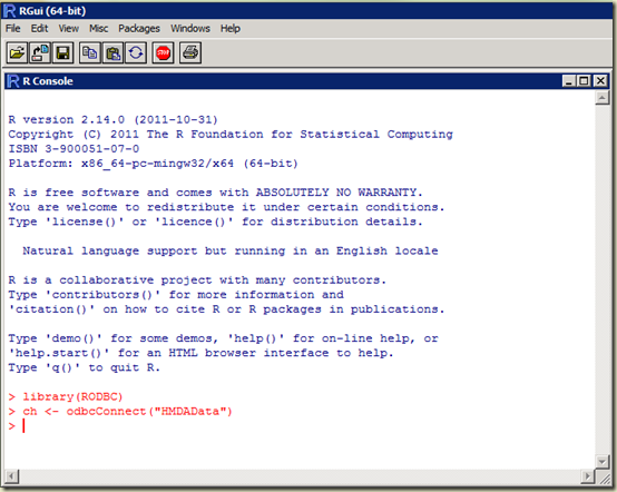
Point to the zip file you just downloaded and R will install the appropriate package and make it available. Once it is available, you can connect to SQL Server by using the following R commands as shown in the figure:

image

Note: R is case sensitive for most operations. Also note that I am entering the commands directly into the R console. Another way to do this is to use the File command and create a new R script, and submit commands from the script to the console. I’ll show this in later posts. Also note that assignment is done in R by using “<-“, this line is basically saying, “assign an object named ‘ch’ to the output of the odbcConnect function that has been passed the value ‘HMDA’”. This will make more sense as you get into R more. What I have done with these commands is load the RODBC library and create a “channel” object that I will use to query SQL Server.

Data Mining with R

In my database, I have a table named “tblIncome” that has 2 columns. Each row is a county in Colorado and the average salary of all people who have applied for a home loan in 2010 within that county. If I wanted to find some “clusters” of salaries within Colorado and see how the income among potential home buyers/refinancers is grouped together, I would take the data and apply K-means clustering techniques to identify the clusters. Normally I’d use SSAS Data Mining, or maybe Excel with the Predixion add-in, but now thanks to R, I can do that analysis directly within R.

The first step is to obtain the data from the SQL Server table and load it into a matrix in R. This can be accomplished using the following command:

image

The “sqlFetch” command simply attaches to a table and does a SELECT * from that table. The “as.matrix” ensures that the data is loaded into a matrix that matches the table structure. You can get a summary of the data with the following command:

image

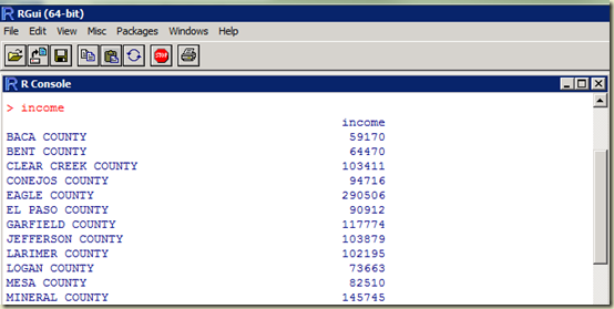
If you just want to see what the income object looks like, you can issue the following command:

image

Now that we have the data loaded into a matrix, we should sort it to make it easier to cluster. Issue the sort command as follows:

image

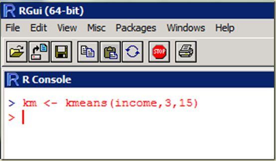
Now that we have the matrix loaded and sorted, we can feed it into the kmeans clustering algorithm. As a note here, anything that you want help with in R you can simply use the ? followed by the command. For example, issue ? kmeans to read all about the kmeans command. For the purposes of this blog entry, I’m just going to use the default algorithm and I’m going to make a guess at 3 clusters to start with and iterate 15 times. I’ll assign the output to the object “km”. The command looks like:

image

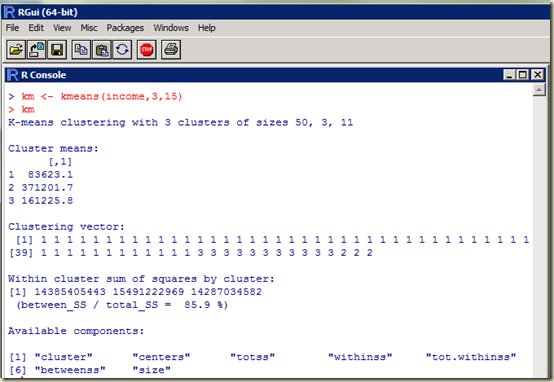
If you want to know what the km object contains, you can issue the following command:

image

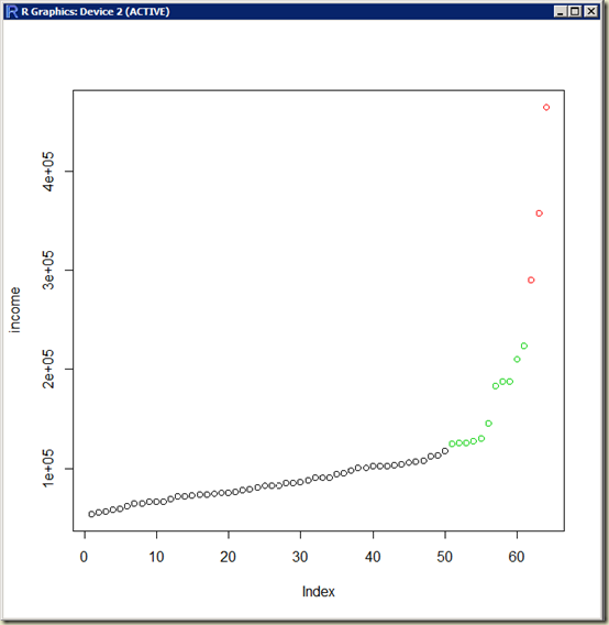
Note that the output has given us 3 clusters with means at 83K, 371K and 161K. We also can see that the object contains various components. To statisticians, this information is very easy to understand, but if you’re like me you probably want to visualize the data. Since I am interested in seeing the cluster associations, I can plot the cluster component. I can use the following command to create the plot:

image

The command generates a plot graph that looks like this:

image

The colors represent our clusters. Since I just guessed that 3 income clusters would be appropriate, the graphic is likely not a very good representation of true income clusters. In order to determine what the true number of clusters should be, I can take the income matrix and compute the sum of squares of each group and determine how many clusters I should have. (You can read about this at http://www.statmethods.net/advstats/cluster.html )

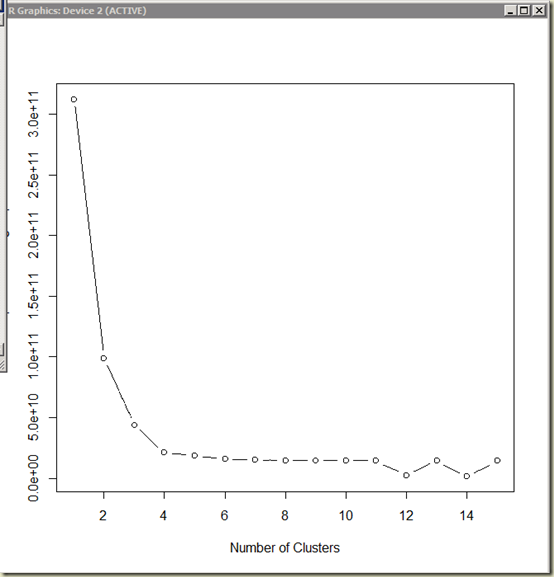
R has the capability of creating loops, so we can iterate through the matrix and plot the resulting sum of squares within the group. We can then plot the results and look for an “elbow” to determine how many clusters would be appropriate with the data that we have. You can accomplish this with the following command:
image

which generates the following plot:

image

which tells us that the appropriate number of clusters is 4.

Conclusion

The intent of this post wasn’t to teach you how to perform statistical analysis using k-means clustering, but rather to demonstrate how some very advanced statistical analysis can be performed from SQL Server data and R without SSAS modeling or advanced Excel use.

Since I am spending a lot of time in the Data Science discipline, I will be posting a lot of R examples using SQL Server data.