Friday, December 30, 2011

Fun with Decision Trees using R and SQL Server

As those who have been reading this blog know, I’ve recently been spending a lot of time doing statistical analysis with R and SQL Server and have really been enjoying digging in to the various bits of functionality that is offered.

One thing I’ve learned over the years is that I am a very “classification-oriented” individual when it comes to working with data. I work best with data sets that I understand and that I’ve been able to sort into the various buckets that make sense to me based on what I’m trying to accomplish with the data.

The problem with this need for nice and tidy data classification is that it doesn’t work well when you don’t really have a complete understanding of the data set you’re working with. This especially becomes an issue if you’re trying to mine the data you have in order to predict future outcomes based on past performance (a requirement that is becoming more and more importing to “Data Scientists” as more and more organizations make that shift to true data-driven processes.

Understanding Data

If you read my previous post on creating a large SQL Server database, you’ve seen some of the data that I am playing around with. Obviously there is a lot of interesting information locked within the mortgage loan application data stored in the HMDA database. One specific use-case with this data might be to look at some of the deciding factors related to home loans being granted and create some predictive models based on the data. For example, I might want to predict the outcome of a home loan application process based on factors like the purpose of the loan, the income of the applicant, and some other factors such as race. This could be very useful for a mortgage company to look at and see who to target for an ad campaign, or maybe to research things such as do race or sex have any correlation to the amount of a home loan given. In order to answer this use case, we need to have a good understanding of the data we’re working with and see what it looks like when shaped into a “Decision Tree” (for more information on what exactly a decision tree is, take a look at: http://en.wikipedia.org/wiki/Decision_tree )

Creating a Data Set to Work With

If we wanted to use the home mortgage disclosure data to look at past performance of home loans, the first thing we need to do is create a manageable data set to use to create a model. Since I live in El Paso County, Colorado, I’ll create a table of data that just details information on Home Loans in this area. Given the database that was created earlier (see previous post) We can create a subset of the data with the following query:

SELECT 
loan_purpose AS [purpose]
,loan_amount AS [amount]
,CASE WHEN applicant_race = 'White' THEN applicant_race ELSE 'Non-White' END AS [race]
,applicant_sex AS [sex]
,applicant_income AS [income]
,CASE WHEN denial_reason = 'Approved' THEN denial_reason ELSE 'Denied' END AS [status]
INTO
tblElPasoCountyLoanStatus
FROM
vColoradoLoans
WHERE county='El Paso County'


What this will do is create a simple table that has 6 columns. I’ve simplified the data slightly so that some of the factors (race, denial reason) are binary values as opposed to continuous. While this is not a necessary transformation for the most part, it helps simplify the output for the purposes of this discussion.


Loading the Appropriate Packages and Libraries in R


Once I’ve created the table above in SQL Server, I can load the data into R and begin analysis. Before we get too deep in the creation of the decision tree, I should mention that I am going to use a package called “rpart” as well as a package called “rpart.plot”. If you are really curious and would like to know the science behind the rpart package, there is a very dry document here that explains the algorithm in detail: http://www.mayo.edu/hsr/techrpt/61.pdf 


The rpart package can be found here: http://cran.stat.ucla.edu/web/packages/rpart/index.html


and rpart.plot can be found here: http://cran.stat.ucla.edu/web/packages/rpart.plot/index.html 


Of course you really don’t need to know where exactly the packages are, you can install them with the R command as follows:


image


When you execute the above command in the R console, you will be prompted for the mirror site you wish to use, and the package will be downloaded, unpacked and installed. Once the packages are installed, you can load them into your R environment as follows:


image


Connecting to SQL Server Data


Once the libraries are loaded, we need to obtain the data we’re going to work with. If you haven’t worked with SQL Server data in R before, you might want to read my previous post on connecting R to SQL Server via the ODBC library. First we need to setup an ODBC channel to connect to the table we created above. Is is done via the following command:


image


(Remember that “HMDAData” is the name of the ODBC DSN I created to connect to my database)


Once the channel is created, I can load the data from the table via the sqlFetch command in R as follows:


image


Examining the Data


This loads the data from the table into the R variable “loanstatus”. You can view a summary of the loanstatus as follows:


image


Already you can see that we’ve extracted some good information out of the database. (as a side note here, I think this is VERY COOL! Think of all the SQL Queries I’d have to run to get this same information from the table I created earlier)


Now that we have the data in an R variable, we can start to create a decision tree. Since we ultimately want to use this data to predict the amount of a loan based on certain factors such as race, sex and income, we’ll create a regression tree shaped to those parameters. We will use the rpart function in order to create the tree. rpart is a very simplistic function that accepts the following parameters:


  • formula – The formula is specified in the following format: outcome ~ predictor1 + predictor2 + predictor3 etc.


  • data – The specific data frame to use


  • method – “class” for a classification tree or “anova” for a regression tree


Remember that within R, you can always type ? <function> to get a full description of a particular function.


In our case, the rpart command would look like this:


image


Once we’ve created the tree variable (this can be named anything, I just kept it simple and named it “tree” here) we can look at a summary and determine what it looks like:


image


(there are a total of 13 nodes in my specific example, and I can’t paste the entire tree here in text form)


One big factor in determining how useful a particular decision tree going to be is to examine the “complexity parameter” (“cp” for short) for each of the nodes. The CP is used to cross-validate the data and make sure that the tree is pruned to remove the portions of the tree that are “over fitted” (You can read about the terminology here: http://www.statmethods.net/advstats/cart.html ) . Since I am a very visual person, I like to see this cross-validation data in chart form as follows:


image


Which generates a nice graph showing me the relative size of the tree, the cross-validated error that is generated, and the resulting cp:


image


Since the tree that I am working with is relatively small, I am not going to worry about pruning it here and removing the “bad” cp values. To generate the decision tree, use the following command:


image


(Remember that you can use the ? command to get a full listing of all options for a given function. In this case, by using type=4 I am instructing R to generate a plot containing all nodes and all information, and by using extra=1 I am instructing R to include the number of nodes in each branch)


image


With this visual of the tree, I can see that income seems to be a deciding factor, and it splits at approximately 90,000. Following the tree to the left, for those with less than 90K income, we see a split for Home Improvement loans versus Home Purchase and refinance. For the purchase and refinance, we see another split at approximately 52K income. Back on the right side of the tree we see a split at approximately 208K income, with the same split for home improvement loans versus purchase and refinance.


Conclusion


Being the data geek that I am, I could continually refine this model and graph it to start finding the patterns and determining just exactly how the data is shaped. At that point I could feed additional data into the model and use it to predict outcomes based on past performance. There are many things that can be done with Decision Trees and I’ve only scratched the surface here with this post. I’ll be writing many more of these posts in the future as I continue to explore the magic of data mining with R.

Wednesday, December 28, 2011

To The Cloud and Back Again! – SQL Saturday # 104

For those that are not aware, the Professional Association for SQL Server (PASS) has chapters throughout the world that put on one day events called “SQL Saturday”. As the name implies, these events take place on a Saturday and generally are a full day of targeted learning for those who want to know more about SQL Server and SQL Server technologies.

This year, the first US SQL Saturday event (There is also an event in Bangalore that same day, and given the time zones, I’d say they qualify as the “first” one of the year!)  is happening right here in Colorado Springs! SQL Saturday #104 has a very distinguished list of speakers, including people like Jason Horner, TJ Belt, Chris Shaw, Thomas LaRock, Karen Lopez and a whole host of very impressive speakers. There’s going to be 5 simultaneous tracks and somehow they even invited me to speak as well, so I’ll be speaking at 0830 in room #4 on “To the Cloud and Back Again!”.

Session Description

In this session, I’ll be introducing some basic Cloud Computing patterns and will talk about some specific cloud computing security concerns. I’ll then talk about some of the specific technologies that accompany the Windows Azure and SQL Azure platforms that enable a hybrid approach to cloud computing. I’ll demonstrate how Windows Azure roles can be “Domain Joined” that will then allow Azure-based applications to use SQL Server Trusted Connections to connect to on-premises SQL Server databases. All in all I hope it will be a very informative session on Cloud Computing technologies. Hope to see you there!

image

Monday, December 26, 2011

Building a large real-world SQL Server demo database

In my previous post, I discussed a large data set that I was using for demonstrations and working with R. Instead of using the normal AdventureWorks or Northwind databases that Microsoft makes available to us via Codeplex, I wanted something a bit more real-world as well as large. I also wanted something that I could continue to build on as more data became available. I had never really found anything that I liked and basically relegated the thought to a background task.

As I mentioned in the last post,  I had the opportunity to attend an alpha delivery of the EMC “Data Science and Big Data Analytics” training course. As we were working through the labs, I couldn’t help but think that the data set being used was very interesting, and would almost fit what I had been looking for. In speaking with the creators of the class, I learned that they had built the database based on information obtained from the publically-available “Home Mortgage Disclosure Act” reporting site. Here in the US, when you apply for a home mortgage loan you must provide certain information to the lending institution, and they in turn must report information on all applications that they process, whether they are approved or denied. The information itself is stripped of personal-identifiers when it is submitted, but the overall type of data that is reported is extremely interesting from both a volume perspective as well as a content perspective. I decided to spend a bit of time looking in to how I could gain access to this data, and thanks to the magic of the interwebs, I was able to piece together everything I needed in order to build the database I was looking for.

Gaining Access to the Home Mortgage Disclosure Act Data

(I realize that the information posted here is really only relevant to those of us in the United States, however I believe the resulting data is useful and relevant worldwide for purposes of learning or demo)

The Home Mortgage Disclosure Act was enacted by Congress in 1975 and is administered by the “Federal Financial Institution Examination Council”. Because it is a government institution and funded by US taxpayer dollars, the data that they collect and maintain is made available to the public free of charge. Basically what they do is chunk the data into yearly “drops” that are made available according to a specific timeline. You can read about the timeline here: http://www.ffiec.gov/hmda/timeline.htm 

The data itself is available from the following link:

http://www.ffiec.gov/hmda/

There are multiple ways to obtain the data for a given year. The easiest way to get to the data is to download the “LAR/TS Windows Application” for a given year. (LAR = “Loan Accounts Register”, TS=”Transmittal Sheet”). You can download the application from the following link: http://www.ffiec.gov/hmda/hmdaproducts.htm (note the Windows application download links towards the bottom of the page). When downloaded, the application contains all of the data for a given year within a SQL Server Compact Edition (SQLCE) database. The database itself is about 5GB per year. Of course the problem with this format is that it’s strictly a SQLCE database, which means you’ll want to extract the data for use with SQL Server. Another issue with the data is that it is organized by a seemingly random collection of states, meaning that there is no single dataset that contains the data within a given year for the entire country.

Another way to obtain the data is to download the text files directly from the site. The files are zipped and can be found by downloading the “ALL” file in the LAR table for the year that you are interested in. (At the time of this posting, there are 3 years available, 2008, 2009 and 2010). These files are tab-delimited and will need to be imported to SQL Server.

Creating the HMDA Database

Because I want to create a database that will have a single “fact” table containing all of the LAR records, I will need to first create the database and then the table structure necessary. The HMDA data is very “flat” and denormalized, so it works very well as a fact table. There are 45 fields contained in the text file and column names are NOT included in the first row. The data dictionary can be found here: LAR Record Format

Since the resulting database will work out to be about 5GB per year, and since we’ll be importing 3 years of data, I’ll start by creating a 15GB database with the following T-SQL(I am using SQL Server 2012 as my destination, so some of the syntax might be slightly different than you are used to) command:

CREATE DATABASE [HMDAData]
CONTAINMENT = NONE
ON  PRIMARY
( NAME = N'HMDAData', FILENAME = N'C:\SQLData\MDF\HMDAData.mdf' , SIZE = 15GB , MAXSIZE = UNLIMITED, FILEGROWTH = 1024MB )
LOG ON
( NAME = N'HMDAData_log', FILENAME = N'C:\SQLData\LDF\HMDAData_log.ldf' , SIZE = 8GB , MAXSIZE = 2048GB , FILEGROWTH = 10%);

Once the database is created, we can create the table to hold the LAR records. The table can be created with the following command:


CREATE TABLE [dbo].[lar_data](
    [year] [int] NOT NULL,
    [respid] [nchar](10) NOT NULL,
    [agycd] [nchar](1) NOT NULL,
    [loan_type] [int] NOT NULL,
    [property_type] [int] NOT NULL,
    [loan_purpose] [nchar](1) NULL,
    [occupancy] [nchar](1) NULL,
    [loan_amount] [nchar](5) NULL,
    [preapproval] [nchar](1) NULL,
    [action_type] [nchar](1) NULL,
    [msa_md] [nchar](5) NULL,
    [state_code] [int] NOT NULL,
    [county_code] [int] NULL,
    [tract_code] [nchar](7) NOT NULL,
    [applicant_ethnicity] [nchar](1) NULL,
    [co_applicant_ethnicity] [nchar](1) NULL,
    [applicant_race_1] [nchar](1) NULL,
    [applicant_race_2] [nchar](1) NULL,
    [applicant_race_3] [nchar](1) NULL,
    [applicant_race_4] [nchar](1) NULL,
    [applicant_race_5] [nchar](1) NULL,
    [co_applicant_race_1] [nchar](1) NULL,
    [co_applicant_race_2] [nchar](1) NULL,
    [co_applicant_race_3] [nchar](1) NULL,
    [co_applicant_race_4] [nchar](1) NULL,
    [co_applicant_race_5] [nchar](1) NULL,
    [applicant_sex] [nchar](1) NULL,
    [co_applicant_sex] [nchar](1) NULL,
    [applicant_income] [nchar](4) NULL,
    [purchaser_type] [nchar](1) NULL,
    [denial_reason_1] [nchar](1) NULL,
    [denial_reason_2] [nchar](1) NULL,
    [denial_reason_3] [nchar](1) NULL,
    [rate_spread] [nchar](5) NULL,
    [HOEPA_status] [nchar](1) NULL,
    [lien_status] [nchar](1) NULL,
    [edit_status] [nchar](1) NULL,
    [seq_number] [nchar](7) NULL,
    [population] [int] NULL,
    [minority_population_percent] [numeric](18, 0) NULL,
    [median_income] [int] NULL,
    [tract_msa_income_percent] [numeric](18, 0) NULL,
    [owner_occ_units] [int] NULL,
    [owner_occ_1_to_4_family] [int] NULL,
    [app_date_pre_2004] [nchar](1) NULL
) ON [PRIMARY];

Once the table is created, you can either use the SQL Server Import/Export wizard or SSIS to import each of the files to the lar_data table. Since it is a simple data load process without any conversions needed, the Import/Export Wizard works just fine. Here’s an example of importing the 2010 file to the lar_data table:

image

image

image


image

Because the text file will contain character data there will be CASTs required for most columns. In the event that an error occurs within a specific CAST, it’s best to just ignore it. We’re not trying to create a perfect database, just one that works for most conditions.

image

image

When the import for 2010 is complete, there will be approximately 16.3 million rows of data inserted into the table.

To complete the task, import the remaining years into the table. You should end up with approximately 53.2 million rows in the table if you copy 2008, 2009 and 2010 data.

You may notice that several of the columns are codes and not well described. You can find the information for each of the columns in the data dictionary linked above, however the data for each of the columns can be a pain to enter. Since I have already extracted the data and created appropriate tables, you can download the following ZIP file (which contains text files that are in .csv format with column names as the first row and the file is named the same as the table it comes from. These files are simple to import using the Import/Export wizard. There is also a .sql file there to create the remaining tables and insert descriptive data):

Zip file containing dimension tables and descriptive data

Creating an Appropriate “State” View

Now that you have the fact table data loaded, and you’ve used the files I’ve supplied to create the dimensional tables, you’ll likely want to create a subset of the data for specific analysis. Since I live in Colorado, I decided to create a view that shows only Colorado data. The view definition is included below, and you can modify it accordingly to isolate the data for the state you are interested in:

CREATE VIEW [dbo].[vColoradoLoans]
AS
SELECT
    lt.description AS [loan_type]
    ,lpt.description AS [property_type]
    ,lp.description AS [loan_purpose]
    ,o.description AS [occupancy_type]
    ,CAST(loan_amount AS money) * 1000 AS [loan_amount]   
    ,p.description AS [preapproval]
    ,at.description AS [action_taken]
    ,s.state_name AS [state]
    ,c.county_name AS [county]
    ,e.description AS [applicant_ethnicity]   
    ,r.description AS [applicant_race]
    ,sx.description AS [applicant_sex]
    ,CAST(applicant_income AS money) * 1000 AS [applicant_income]   
    ,pt.description AS [purchaser_type]
    ,dr.description AS [denial_reason]
    ,CASE WHEN rate_spread = 'NA' then 0 ELSE CAST(rate_spread AS numeric) END AS [rate_spread]    
    ,population AS [tract_population]
    ,minority_population_percent
    ,median_income
    ,owner_occ_units
FROM
    lar_data ld
JOIN
    tblLoanType lt
ON
    ld.loan_type = lt.loan_type
JOIN
    tblPropertyType lpt
ON
    ld.property_type = lpt.property_type
JOIN
    tblLoanPurpose lp
ON
    ld.loan_purpose = lp.loan_purpose
JOIN
    tblOwnerOccupancy o
ON
    ld.occupancy = o.owner_occupancy
JOIN
    tblPreapproval p
ON
    ld.preapproval = p.preapproval
JOIN
    tblAction at
ON
    ld.action_type = at.action_taken
JOIN
    tblState s
ON
    ld.state_code = s.state_code
JOIN
    tblCounty c
ON
    ld.county_code = c.county_code AND s.state_name=c.state_name
JOIN
    tblEthnicity e
ON
    ld.applicant_ethnicity = e.ethnicity
JOIN
    tblRace r
ON
    ld.applicant_race_1 = r.race
JOIN
    tblSex sx
ON
    ld.applicant_sex = sx.sex
JOIN
    tblPurchaserType pt
ON
    ld.purchaser_type = pt.purchaser_type
JOIN
    tblDenialReason dr
ON
    ld.denial_reason_1 = dr.reason
WHERE
    ld.state_code = '08' -- Colorado
AND
    ld.property_type = 1 -- Single Family Homes
AND
    ld.applicant_income <> 'NA' -- remove invalid income reports
;

Conclusion

Once you have the view in place, you now have a very flexible large database that you can use that has a real-world use-case and can be used for demos, performance tuning work, statistical analysis, etc.. Of course you’ll want to add your own indexes and possibly partitions depending on your use case.

image

I know that I’ve often wanted such a database when presenting or demonstrating specific functions within SQL Server, so I hope this database proves useful.

Friday, December 23, 2011

Statistical Analysis with R and Microsoft SQL Server 2012

It’s been awhile since I’ve written a blog post, but that doesn’t mean that I haven’t been thinking about things to write about and discuss here. Recently, I had the opportunity to attend an alpha delivery of EMCs “Data Science and Big Data Analytics” course (Read about the course on EMC Education Services site here: http://education.emc.com/guest/campaign/data_science.aspx ) and was really taken by a couple of points that the course brought home:

1) There’s much more to statistical analysis than I had ever thought about. (Being a Microsoft SQL Server and Microsoft BI Stack kinda guy, I always figured that you needed Excel and SSAS to do real statistical analysis.

2) Big Data Analytics is a really cool technology discipline!

The course itself was based on the EMC Greenplum Database (Community Edition, which you can download and use for free!) which is an amazing piece of technology (I am very impressed with it’s feature/functionality and integration with things like Hadoop for real parallel computing capabilities) as well as the open source “R” statistical analysis language.

R logo

While it’s true that my role at EMC means that I focus more on the non-Microsoft stack these days, that doesn’t stop me from thinking about how I can apply things that I lean to the Microsoft platform. With that in mind, one of the things that I kept coming back to in the class was, “How would I do this using SQL Server?" As it turns out using R with SQL Server isn’t all that difficult, and it really does open up an entirely new way of thinking about statistical analysis (for me anyway)

R and Statistical Analysis

R is an open source “software environment” that is used primarily for statistical analysis. A huge part of “Data Science” is of course statistical analysis, so the two go hand-in-hand. One very cool aspect of R is the fact that the graphics environment is “built in” (I put that in quotes because R is very modular and requires you to load packages for just about anything you do, although a basic “plot” command is included in the base distribution) and allows you not only to analyze data, but also visualize it “on the fly” as well. You can read about (and download) R from the main website here: http://www.r-project.org/. If you are really interested in R, you should make a point of reading the R Journal here: http://journal.r-project.org/current.html 

One thing that is very clear though about R is that it’s a “data source agnostic” environment, but many of the examples that use data either deal with flat files or connect to open source databases like MySQL or Postgres. This of course doesn’t mean you can’t use R with SQL Server, it just means you have to dig a little deeper and understand how to connect the R environment to your SQL Server database.

R and SQL Server

Once you download and install the R environment (the screen shots and examples I provide here will be from the Windows version of RGUI version 2.14.0 which I downloaded from the UC Berkeley mirror here: http://cran.cnr.berkeley.edu/ ) you will need to install the RGUI environment and decide whether you will use the 32 or 64-bit client. This is a very important distinction, since R connects to databases via ODBC, and ODBC drivers are very platform (32 versus 64 bit) specific.

In my case, I am going to use the 64 bit GUI and will be using SQL Native Client 11 to connect to SQL Server 2012. (There is no specific reason for me to use SQL Server 2012 here, other than I’ve been playing around with the release candidate and my development environment is all setup for it) I have a large database that I use for “big data” type demonstrations that also works well for statistical analysis work. I will likely write another article on how this database was constructed, but know that the data is very real world (it is built from 2010 data collected via the US Home Mortgage Disclosure Act) and well-suited for testing statistical analysis theories and data mining.

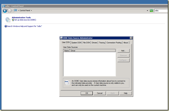
Once you decide what client you will be using, you will need to configure an ODBC DSN (I decided to use a System DSN for my work, so I’ll walk though the creation of that DSN) to connect to your database. To create a new DSN, use the platform-specific version of the ODBC control panel (for Windows Server 2008 R2, simply go to control panel and search for “ODBC”, you will then see the “Set up data sources (ODBC)” as shown in the following figure:

image

Click the “System DSN” tab, and then click the Add button and walk through the wizard to connect to your database. Remember the name of the DSN you create, as you’ll need to specify it from within R in order to connect. In my case, the DSN is named “HMDAData”.

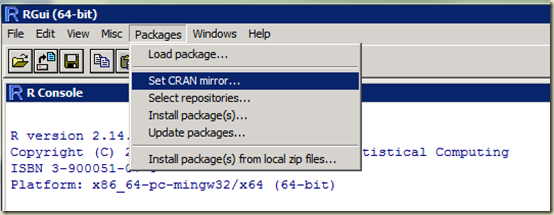
In order to use the ODBC connection within R, you’ll need to download the “RODBC” library, which can be found here: http://cran.cnr.berkeley.edu/web/packages/RODBC/index.html. Select the appropriate zip file and download it to a folder on the machine where you installed R. Once it is downloaded, from within the RGUI, select Packages, and then select “Install packages from local ZIP file” as shown in the following figure:

image

Point to the zip file you just downloaded and R will install the appropriate package and make it available. Once it is available, you can connect to SQL Server by using the following R commands as shown in the figure:

image

Note: R is case sensitive for most operations. Also note that I am entering the commands directly into the R console. Another way to do this is to use the File command and create a new R script, and submit commands from the script to the console. I’ll show this in later posts. Also note that assignment is done in R by using “<-“, this line is basically saying, “assign an object named ‘ch’ to the output of the odbcConnect function that has been passed the value ‘HMDA’”. This will make more sense as you get into R more. What I have done with these commands is load the RODBC library and create a “channel” object that I will use to query SQL Server.

Data Mining with R

In my database, I have a table named “tblIncome” that has 2 columns. Each row is a county in Colorado and the average salary of all people who have applied for a home loan in 2010 within that county. If I wanted to find some “clusters” of salaries within Colorado and see how the income among potential home buyers/refinancers is grouped together, I would take the data and apply K-means clustering techniques to identify the clusters. Normally I’d use SSAS Data Mining, or maybe Excel with the Predixion add-in, but now thanks to R, I can do that analysis directly within R.

The first step is to obtain the data from the SQL Server table and load it into a matrix in R. This can be accomplished using the following command:

image

The “sqlFetch” command simply attaches to a table and does a SELECT * from that table. The “as.matrix” ensures that the data is loaded into a matrix that matches the table structure. You can get a summary of the data with the following command:

image

If you just want to see what the income object looks like, you can issue the following command:

image

Now that we have the data loaded into a matrix, we should sort it to make it easier to cluster. Issue the sort command as follows:

image

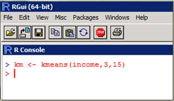
Now that we have the matrix loaded and sorted, we can feed it into the kmeans clustering algorithm. As a note here, anything that you want help with in R you can simply use the ? followed by the command. For example, issue ? kmeans to read all about the kmeans command. For the purposes of this blog entry, I’m just going to use the default algorithm and I’m going to make a guess at 3 clusters to start with and iterate 15 times. I’ll assign the output to the object “km”. The command looks like:

image

If you want to know what the km object contains, you can issue the following command:

image

Note that the output has given us 3 clusters with means at 83K, 371K and 161K. We also can see that the object contains various components. To statisticians, this information is very easy to understand, but if you’re like me you probably want to visualize the data. Since I am interested in seeing the cluster associations, I can plot the cluster component. I can use the following command to create the plot:

image

The command generates a plot graph that looks like this:

image

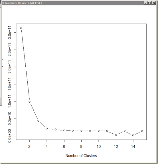
The colors represent our clusters. Since I just guessed that 3 income clusters would be appropriate, the graphic is likely not a very good representation of true income clusters. In order to determine what the true number of clusters should be, I can take the income matrix and compute the sum of squares of each group and determine how many clusters I should have. (You can read about this at http://www.statmethods.net/advstats/cluster.html )

R has the capability of creating loops, so we can iterate through the matrix and plot the resulting sum of squares within the group. We can then plot the results and look for an “elbow” to determine how many clusters would be appropriate with the data that we have. You can accomplish this with the following command:

image

which generates the following plot:

image

which tells us that the appropriate number of clusters is 4.

Conclusion

The intent of this post wasn’t to teach you how to perform statistical analysis using k-means clustering, but rather to demonstrate how some very advanced statistical analysis can be performed from SQL Server data and R without SSAS modeling or advanced Excel use.

Since I am spending a lot of time in the Data Science discipline, I will be posting a lot of R examples using SQL Server data.

Friday, July 8, 2011

Big (say it with me now) Data

Over the last few months I’ve been working with more and more people who have the buzz-phrase, “Big Data” on their minds. For some reason, many people think that “Big Data” (in this context, I’m referring to “Big Data Analytics”) has magical powers and doesn’t require the same careful planning and modeling process that traditional analytics does.


Let’s go ahead and put this thought to rest now. “Big Data” is still “Data” and the data model will make or break your project. The Data Architect (note that I didn’t say “Data Scientist”, that’s a bit different and we’ll get into that in a later post) is still a key position on any Big Data project, and as a matter of fact due to the overwhelming amount of data that is crunched, analyzed and stored, the Data Architect is likely your most important asset.


It is very true that traditional, narrowly-focused data modeling techniques will not work in the Big Data world. Data Architects working with Big Data must understand that Big Data requires thought on an entirely new dimension (forgive the pun) in the modeling of data structures. Not only must you consider the traditional modeling of relationships, structures and indexes, you must also understand how parallel processing will impact your queries, how data will be loaded in partitioned systems, and how adding new nodes into a Big Data cluster will impact existing data models. These are new skills that Data Architects who plan to work with Big Data must learn.

Friday, July 1, 2011

Microsoft MVP for another year!

Was honored to receive “the email” from the Microsoft MVP Award Program letting me know that I have been awarded MVP for another year in Visual Studio ALM. Have to say that I am very honored to be a part of this program!

The upcoming year will be a very good one for ALM folks, and I think those of us with a data focus will especially be happy with new and improved tools.

Thanks Microsoft!

Thursday, June 30, 2011

The Cloud and Software Engineering

In my role here at EMC, I have the opportunity to speak to many of our software development teams about how software development is changing. One of the presentations that I give discusses industry trends that are impacting the way we think about designing and developing software. In that particular presentation, there’s a rather boring graphic that looks like this:

image

This graphic represents the fact that “the cloud” is an important concept that software developers (especially those of us working in the IT Infrastructure management realm) need to be aware of and need to understand.

How “The Cloud” Impacts Software Engineering

Many people would argue that “The Cloud” (be it a private cloud, a public cloud or a hybrid) doesn’t really change anything about how software is engineered since it’s all about infrastructure, and after all, infrastructure is not the concern of the software engineer, right? The problem with that mode of thinking is that one big promise of the cloud movement is flexibility, and software that runs “in the cloud” needs to embrace that flexibility. Consider these points:

  1. Cloud offerings billing themselves as “Platform as a Service (PaaS)” generally attempt to abstract the physical hardware environment from the virtualized application platform that software is built on. At a very high level, what this means is that developers who build applications for PaaS offerings don’t have any control over how the hardware is configured, maintained and protected.
  2. Cloud offerings billing themselves as “Infrastructure as a Service (IaaS)” generally provide a the ability for hosting of virtual machines that are fully-controlled by the customer, but like PaaS offerings, abstract the physical implementation and associated maintenance from the customer.

In both cases above, software engineers need to understand that the environment that their software is executing on is subject to change without notice. In the case of PaaS offerings, developers need to think about persistent storage and volatile storage rather than simply writing to disk. For example, consider an normal application that writes data to a storage device. In many cases, the developer would choose to write that data to a logical disk hosted by the server that the application is executing on. The issue here is that for PaaS, in most cases the “disk” storage available to your application is volatile in nature and in the event that the environment hosting your app changes (failover, patch maintenance, network maintenance, etc) the state of the “disk” is not guaranteed, so for data that must be persisted, developers need to create and maintain non-volatile storage. In the case of IaaS offerings, in the event of a failover or other need to move the hosted virtual machine, there is no guarantee that the state of the VM will be maintained (i.e., it’s possible that the VM could be reset to its initial state, and thus developers need to consider building in mechanisms to deal with that possibility.

The point of the above is that software engineers need to consider the inherit flexibility requirements of the cloud infrastructure when designing and building software that is deployed “to the cloud”.

Wednesday, June 29, 2011

SQL Server Worldwide User Group (SSWUG) PowerPivot Analytics Expo

The folks at SSWUG are putting on a PowerPivot Analytics expo on July 15th. I’ll be speaking at the event on “SharePoint 2010 Business Intelligence Feature Review”. My session will be broadcast from 11:30am – 1:00pm Mountain Daylight Time. The session will cover Excel Services, and how it fits into the larger Business Intelligence ecosystem for SharePoint 2010. I will also be covering an introduction to PowerPivot and how it helps to deliver “BI for the masses” when coupled with SharePoint as a delivery mechanism.


These expos are designed to give people a one day seminar of focused content, and also introduces the Virtual Conference system, which works very well. People can sit at their desks and still have that “going to a technical conference” feeling.

Check it out! To learn more and to register for the event, see http://www.vconferenceonline.com/event/home.aspx?id=281

Moving the Blog Back Here!

Well, after playing around with the blog on my local server, I’ve decided that it really does work best here on blogger. I have changed the url to http://blog.sqltrainer.com so hopefully that won’t confuse things too much.


I always say this, but I’m hoping to spend more time blogging about stuff here over the next year. Work has been exceptionally exciting and I’ve had the awesome opportunity to work with some very cool technologies that I’d love to spend more time educating others about. Time is always an issue though, so we’ll see how it goes.

Thursday, January 6, 2011

Moving the Blog to a New Home

Blogger has been very good to me for this blog, but I am moving it to a new home on my personal website. I’ve been playing around with the incredibly functional mojoPortal (check it out, it’s VERY cool) for my website and the blog technology seems very useful, so I’m going to start using that platform instead.

Check it out: Business Intelligence and Agile Development blog on SQLTrainer.com.